Characterize batch effects
Almut Lütge
19 April, 2020
csf_media
suppressPackageStartupMessages({
  library(CellBench)
  library(scater)
  library(CellMixS)
  library(variancePartition)
  library(purrr)
  library(jcolors)
  library(here)
  library(tidyr)
  library(dplyr)
  library(stringr)
  library(ComplexHeatmap)
  #library(ggtern)
  library(gridExtra)
  library(scran)
  library(cowplot)
  library(CAMERA)
  library(ggrepel)
  library(readr)
})

options(bitmapType='cairo')
Dataset and parameter
sce <- readRDS(params$data)

param <- readRDS(params$param)
celltype <- param[["celltype"]]
batch <- param[["batch"]]
sample <- param[["sample"]]
dataset_name <- param[["dataset_name"]]
dataset_name
## [1] "csf_media"n_genes <- nrow(sce)
table(colData(sce)[,celltype])##
## 0 1 2 3 4
## 2005 794 149 148 53table(colData(sce)[,batch])##
## cryo fresh
## 2370 779res_de <- readRDS(params$de)
abund <- readRDS(params$abund)
outputfile <- params$out_file
cols <-c(c(jcolors('pal6'),jcolors('pal8'))[c(1,8,14,5,2:4,6,7,9:13,15:20)],jcolors('pal4'))
names(cols) <- c()Visualize data
How are sample, celltypes and batches distributed within normalized, but not batch corrected data?
feature_list <- c(batch, celltype, sample)
feature_list <- feature_list[which(!is.na(feature_list))]

lapply(feature_list, function(feature_name){
  visGroup(sce, feature_name, dim_red= "UMAP")
})
## [[1]]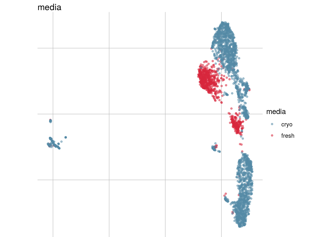
##
## [[2]]
##
## [[3]]
Batch strength/size
To compare or describe the severity of a batch effect there are different meassures. In general they can either give an estimate of the relative strength compared to the signal of interest e.g. the celltype signal or an absolut estimate e.g. the number of batch affected genes.
Variance partitioning
How much of the variance within the datasets can we attributed to the batch effect and how much could be explained by the celltype? Which genes are mostly affected?
vp_vars <- c("vp_batch", "vp_celltype", "vp_residuals")
vp <- as_tibble(rowData(sce)[, vp_vars])  %>% dplyr::mutate(gene= rownames(sce)) %>% dplyr::arrange(-vp_batch)
vp_sub <- vp[1:3] %>% set_rownames(vp$gene)
## Warning: Setting row names on a tibble is deprecated.#plot
plotPercentBars( vp_sub[1:10,] )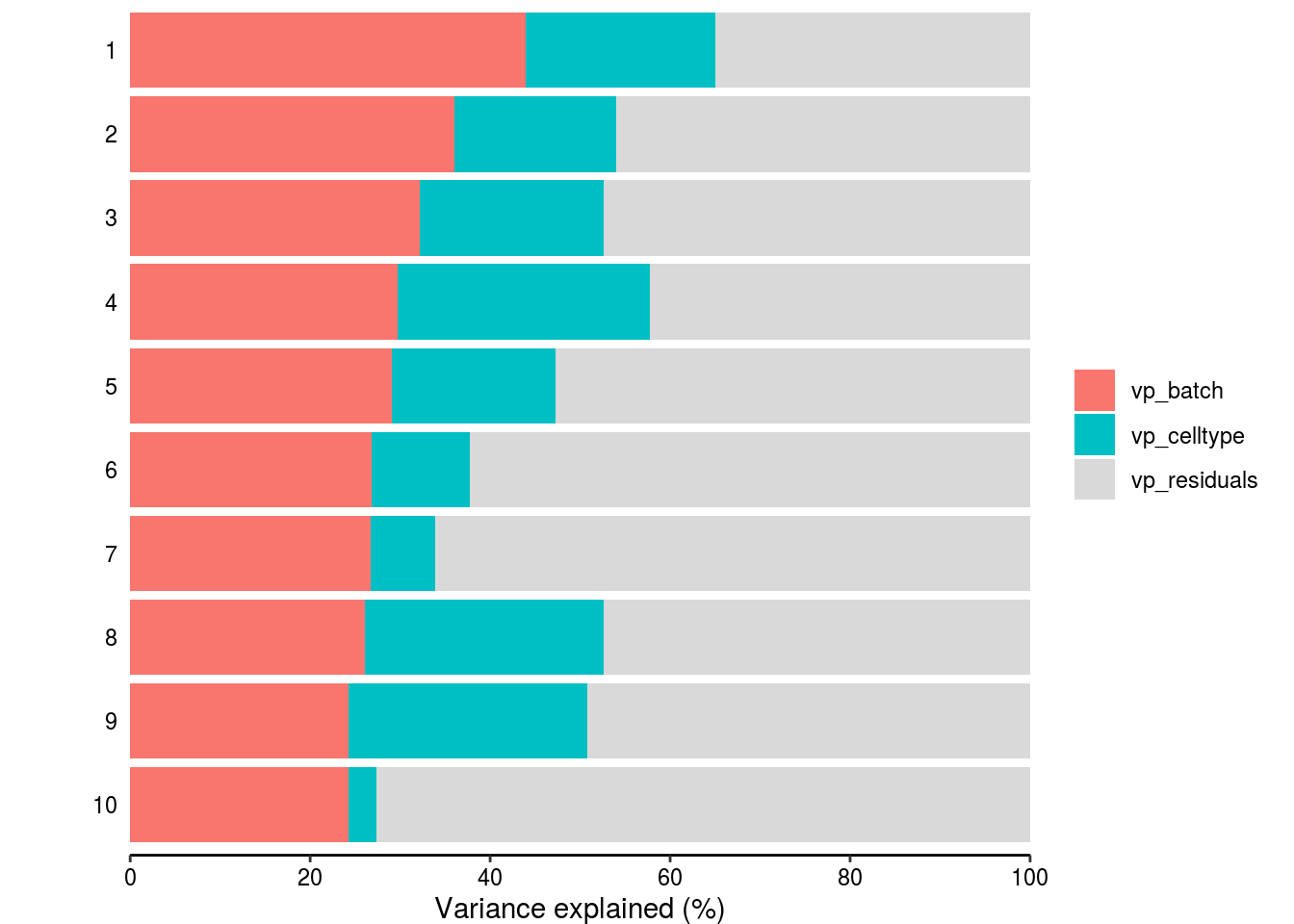
plotVarPart( vp_sub )
Variance and gene expression
Are general expression and batch effect related? Does the batch effect or the celltype effect preferable manifest within highly, medium or low expressed genes?
#define expression classes by mean expression quantiles
th <- quantile(rowMeans(assays(sce)$logcounts), c(.33, .66))
high_th <- th[2]
mid_th <- th[1]

rowData(sce)$expr_class <- ifelse(rowMeans(assays(sce)$logcounts) > high_th, "high",
                                  ifelse(rowMeans(assays(sce)$logcounts) <= high_th &
                                           rowMeans(assays(sce)$logcounts) > mid_th,
                                         "medium", "low"))
rowData(sce)$mean_expr <- rowMeans(assays(sce)$logcounts)

#plot
plot_dev <- function(var, var_col){
  ggplot(as.data.frame(rowData(sce)), aes_string(x = "mean_expr", y = var, colour = var_col)) +
  geom_point() +
  geom_smooth(method = "lm", se = FALSE)
}

#Ternary plots
# ggtern(data=as.data.frame(rowData(sce)),aes(vp_batch, vp_celltype, vp_residuals)) +
#   stat_density_tern(aes(fill=..level.., alpha=..level..),geom='polygon') +
#   scale_fill_gradient2(high = "red") +
#   guides(color = "none", fill = "none", alpha = "none") +
#   geom_point(size= 0.1, alpha = 0.5)  +
#   Llab("batch") +
#   Tlab("celltype") +
#   Rlab("other") +
#   theme_bw()
#
# t1 <- ggtern(data=as.data.frame(rowData(sce)),aes(vp_batch, vp_celltype, vp_residuals)) +
#   geom_point(size = 0.1) +
#   geom_density_tern() +
#   Llab("batch") +
#   Tlab("celltype") +
#   Rlab("other") +
#   theme_bw()

## Summarize variance partitioning
# How many genes have a variance component affected by batch with > 1%
n_batch_gene <- vp_sub %>% dplyr::filter(vp_batch > 0.01) %>% nrow()/n_genes
n_batch_gene10 <- vp_sub %>% dplyr::filter(vp_batch > 0.1) %>% nrow()/n_genes
n_celltype_gene <- vp_sub %>% dplyr::filter(vp_celltype> 0.01) %>% nrow()/n_genes
n_rel <- n_batch_gene/n_celltype_gene

# Mean variance that is explained by the batch effect/celltype
m_batch <- mean(vp_sub$vp_batch, na.rm = TRUE)
m_celltype <- mean(vp_sub$vp_celltype, na.rm = TRUE)
m_rel <- m_batch/m_celltype
Scatterplot batch
plot_dev("vp_batch", "vp_batch")## `geom_smooth()` using formula 'y ~ x'
Scatterplot celltype
plot_dev("vp_celltype", "vp_celltype")## `geom_smooth()` using formula 'y ~ x'
Ternary plot all genes
#t1Ternary plot gene expression classes
#t1 + facet_grid(~expr_class)Cellspecific Mixing score
Overall
#visualize overall cms score
visHist(sce, n_col = 2, prefix = FALSE)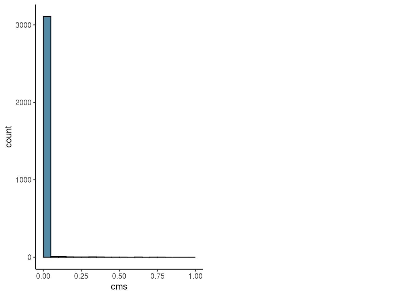
visMetric(sce, metric = "cms_smooth", dim_red = "UMAP")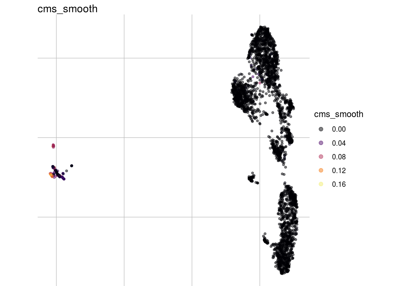
visGroup(sce, celltype, dim_red = "UMAP")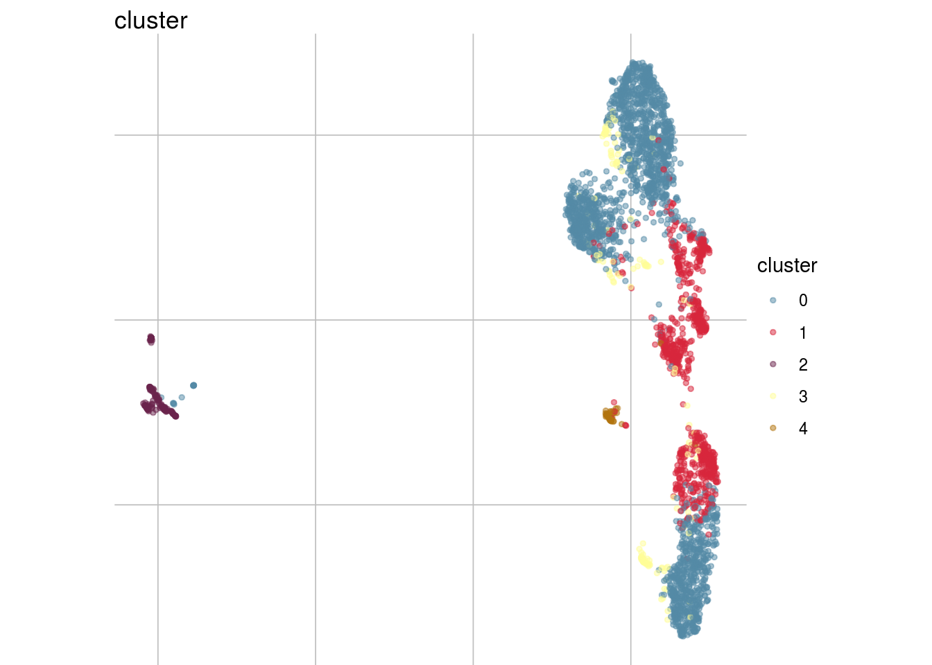
#summarize
mean_cms <- mean(sce$cms)
n_cms_0.01 <- length(which(sce$cms < 0.01))
cluster_mean_cms <- as_tibble(colData(sce)) %>% group_by_at(celltype) %>% summarize(cms_mean = mean(cms))
var_cms <- var(cluster_mean_cms$cms_mean)
Celltypes cms smooth
#compare by celltypes
visCluster(sce, metric_var = "cms_smooth", cluster_var = celltype)
## Picking joint bandwidth of 0.00304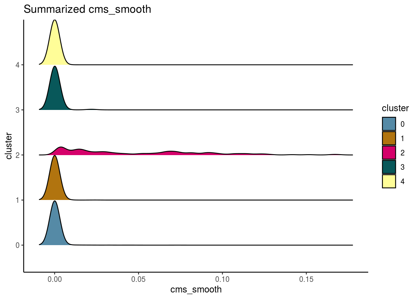
visCluster(sce, metric_var = "cms_smooth", cluster_var = celltype, violin = TRUE)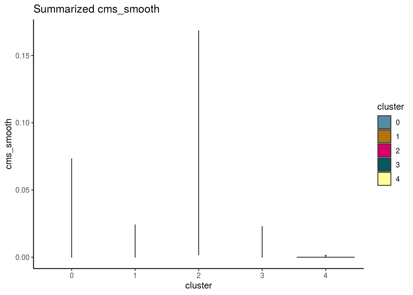
Celltypes histogram
#compare histogram by celltype

p <- ggplot(as.data.frame(colData(sce)),
            aes_string(x = "cms", fill = celltype)) +
                geom_histogram() +
                facet_wrap(celltype, scales = "free_y", ncol = 3) +
                scale_fill_manual(values = cols) +
                theme_classic()

p + geom_vline(aes_string(xintercept = "cms_mean",
                   colour = celltype),
               cluster_mean_cms, linetype=2) +
  scale_color_manual(values = cols)
## `stat_bin()` using `bins = 30`. Pick better value with `binwidth`.
Celltype specificity
Celltype abundance
meta_tib <- as_tibble(colData(sce)) %>% group_by_at(c(batch, celltype)) %>% summarize(n = n()) %>% dplyr::mutate(cell_freq = n / sum(n))

plot_abundance <- function(cluster_var, tib, x_var){
  meta_df <- as.data.frame(eval(tib))
  p <- ggplot(data=meta_df, aes_string(x=x_var, y="cell_freq", fill = cluster_var)) +
    geom_bar(stat="identity") + scale_fill_manual(values=cols, name = "celltype")
  p + coord_flip() + theme_minimal()
}

plot_abundance(cluster_var = celltype, tib = meta_tib, x_var = batch)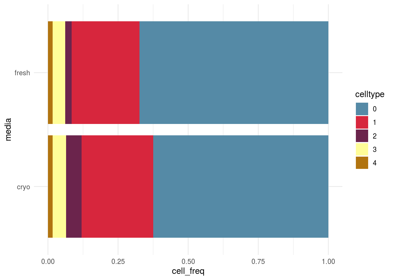
#summarize diff abundance
mean_rel_abund_diff <- mean(unlist(abund))
min_rel_abund_diff <- min(unlist(abund))
max_rel_abund_diff <- max(unlist(abund))
Batch and celltype specific count distributions
Do the overall count distribution vary between batches? Are count distributions celltype depended
#batch level
bids <- levels(as.factor(colData(sce)[, batch]))
names(bids) <- bids
cids <- levels(as.factor(colData(sce)[, celltype]))
names(cids) <- cids

#mean gene expression by batch and cluster
mean_list <- lapply(bids, function(batch_var){
  mean_cluster <- lapply(cids, function(cluster_var){
    counts_sc <- as.matrix(logcounts(
      sce[, colData(sce)[, batch] %in% batch_var &
            colData(sce)[, celltype] %in% cluster_var]))
  })
  mean_c <- mean_cluster %>% map(rowMeans) %>% bind_rows %>%
    dplyr::mutate(gene=rownames(sce)) %>%
    gather(cluster, logcounts, cids)
})
## Note: Using an external vector in selections is ambiguous.
## ℹ Use `all_of(cids)` instead of `cids` to silence this message.
## ℹ See <https://tidyselect.r-lib.org/reference/faq-external-vector.html>.
## This message is displayed once per session.mean_expr <- mean_list %>% bind_rows(.id= "batch")
ggplot(mean_expr, aes(x=logcounts, colour=batch)) + geom_density(alpha=.3) +
theme_classic() +
facet_wrap( ~ cluster, ncol = 3) +
scale_colour_manual(values = cols) +
scale_x_continuous(limits = c(0, 7))## Warning: Removed 8 rows containing non-finite values (stat_density).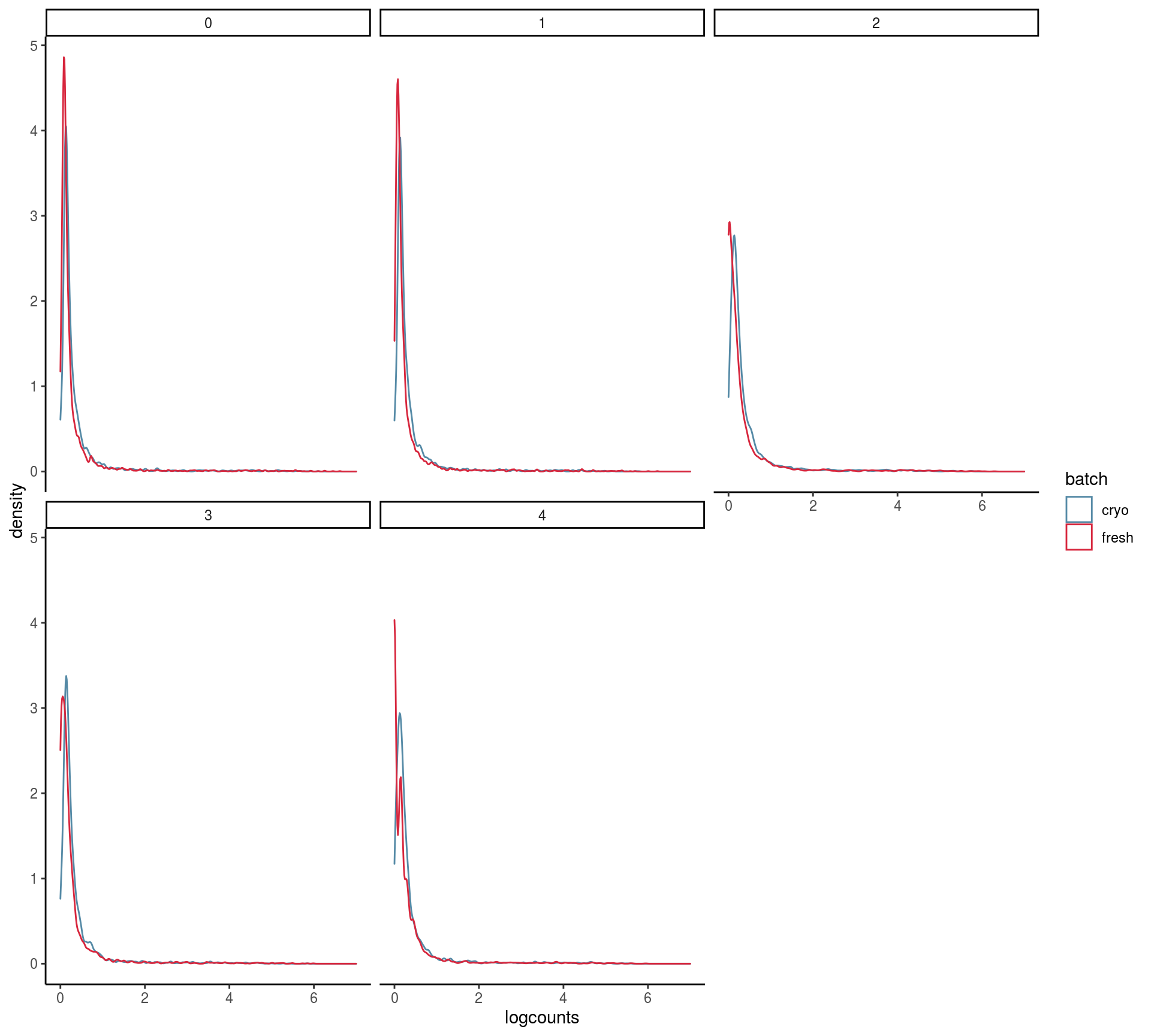
Batch to batch comparisons of expression distributions
Differentially expressed genes
Upset plot
## Upset plot\
cont <- param[["cont"]]
cs <- names(cont)
names(cs) <- cs

# Filter DEG by pvalue
FilterDEGs <- function (degDF = df, filter = c(FDR = 5)){
  rownames(degDF) <- degDF$gene
  #pval <- degDF[, grep("adj.P.Val$", colnames(degDF)), drop = FALSE]
  pval <- degDF[, grep("PValue$", colnames(degDF)), drop = FALSE]
  pf <- pval <= filter["FDR"]/100
  pf[is.na(pf)] <- FALSE
  DEGlistUPorDOWN <- sapply(colnames(pf), function(x) rownames(pf[pf[, x, drop = FALSE], , drop = FALSE]), simplify = FALSE)
}

result <- list()
m2 <- list()

for(jj in 1:length(cs)){
  result[[jj]] <- sapply(res_de[[1]][[names(cs)[jj]]], function(x) FilterDEGs(x))
  names(result[[jj]]) <- cids
  m2[[jj]] = make_comb_mat(result[[jj]], mode = "intersect")
}

names(result) <- names(cs)
names(m2) <- names(cs)

lapply(m2, function(x) UpSet(x))
## $`cryo-fresh`
Logfold_change and GSEA
# DE genes (per cluster and mean)
res <- res_de[["table"]]
#n_de <- lapply(res, function(y) vapply(y, function(x) sum(x$adj.P.Val < 0.05), numeric(1)))
n_de <- lapply(res, function(y) vapply(y, function(x) sum(x$adj.PValue < 0.05), numeric(1)))
n_genes_lfc1 <- lapply(res, function(y) vapply(y, function(x) sum(abs(x$logFC) > 1), numeric(1)))
mean_n_genes_lfc1 <- mean(unlist(n_genes_lfc1))/n_genes

# plot DE for all comparison and check gene sets
#get geneset
gs <- read_delim(params$gs, delim = "\n", col_names = "cat")
## Parsed with column specification:
## cols(
## cat = col_character()
## )cats <- sapply(gs$cat, function(u) strsplit(u, "\t")[[1]][-2],
USE.NAMES = FALSE)
names(cats) <- sapply(cats, .subset, 1)
cats <- lapply(cats, function(u) u[-1])
plotDE <- function(cont_var){
#res_s <- res[[cont_var]] %>% map(filter, adj.P.Val < .05) %>% map(filter, abs(logFC) > 1)
res_s <- res[[cont_var]] %>% map(dplyr::filter, PValue < .05) %>% map(dplyr::filter, abs(logFC) > 1)
#plot
lapply(names(res[[cont_var]]), function(ct){
ct_de <- res[[cont_var]][[ct]]
ct_de$gene <- gsub('[A-z0-9]*\\.', '', ct_de$gene)
res_s[[ct]]$gene <- gsub('[A-z0-9]*\\.', '', res_s[[ct]]$gene)
#p <- ggplot(ct_de, aes(x = AveExpr, y = logFC, colour = abs(logFC) > 1, label = gene)) +
p <- ggplot(ct_de, aes(x = logCPM, y = logFC, colour = abs(logFC) > 2, label = gene)) +
geom_point(size = 2, alpha = .5) +
geom_label_repel(data = res_s[[ct]]) +
ggtitle(paste0(ct,": ", cont_var)) +
theme_classic()
print(p)
cat("Cluster:", ct, "Contrast:", cont_var,
"Num genes:", nrow(ct_de), "Num DE:", nrow(res_s[[ct]]), "\n" )
# run 'camera' for this comparison
inds <- ids2indices(cats, ct_de$gene)
#cm <- cameraPR(ct_de$t, inds) #LR
cm <- cameraPR(ct_de$F, inds)
print(cm %>% rownames_to_column("category") %>%
filter(FDR < .05 & NGenes >= 5) %>% head(8))
})
}
if( length(names(res)) <= 3 ){
pathways <- lapply(names(res), plotDE)
}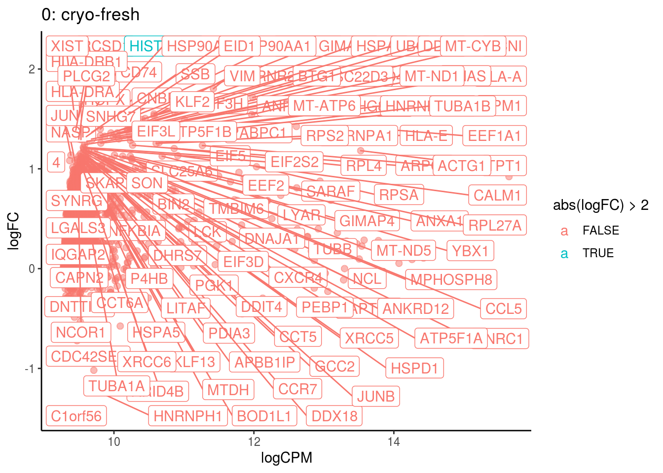
## Cluster: 0 Contrast: cryo-fresh Num genes: 3613 Num DE: 114
##                                     category NGenes Direction       PValue
## 1                            GO_TRNA_BINDING      7        Up 2.206823e-37
## 2  GO_TRANSLATION_ELONGATION_FACTOR_ACTIVITY      7        Up 1.998975e-33
## 3      GO_STRUCTURAL_CONSTITUENT_OF_RIBOSOME    145        Up 1.643518e-22
## 4                            GO_RRNA_BINDING     37        Up 1.435873e-16
## 5            GO_STRUCTURAL_MOLECULE_ACTIVITY    221        Up 1.176031e-14
## 6 GO_TRANSLATION_FACTOR_ACTIVITY_RNA_BINDING     44        Up 6.301742e-07
## 7        GO_FIBROBLAST_GROWTH_FACTOR_BINDING      7        Up 5.077510e-05
## 8                 GO_PEPTIDE_ANTIGEN_BINDING     15        Up 5.993318e-05
##            FDR
## 1 1.825043e-34
## 2 8.265761e-31
## 3 4.530631e-20
## 4 2.374934e-14
## 5 1.620963e-12
## 6 6.514426e-05
## 7 4.665667e-03
## 8 4.956474e-03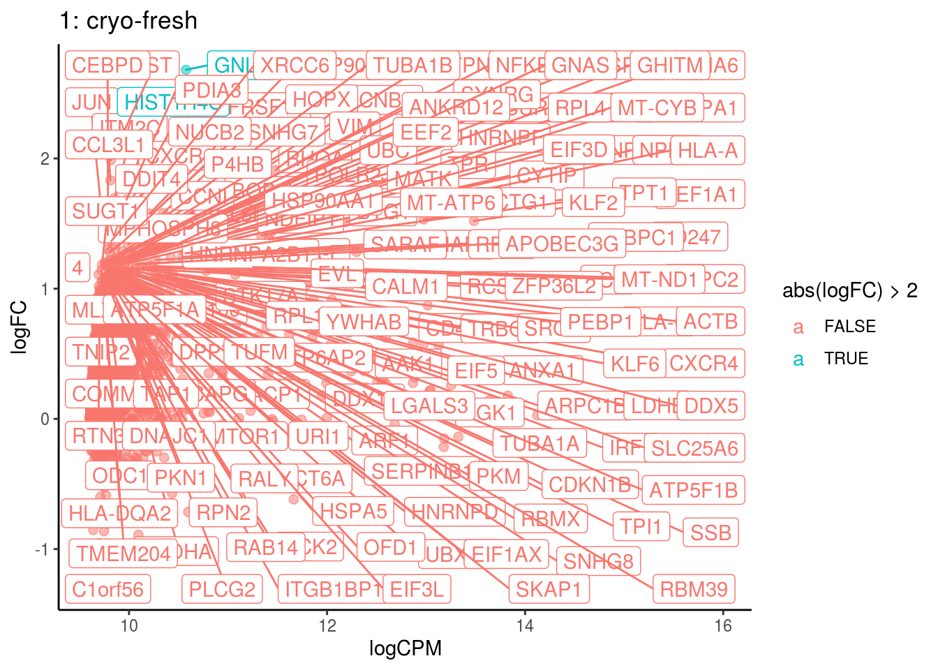
## Cluster: 1 Contrast: cryo-fresh Num genes: 3613 Num DE: 142
##                                    category NGenes Direction       PValue
## 1 GO_TRANSLATION_ELONGATION_FACTOR_ACTIVITY      7        Up 2.914633e-32
## 2                           GO_TRNA_BINDING      7        Up 2.865378e-30
## 3     GO_STRUCTURAL_CONSTITUENT_OF_RIBOSOME    145        Up 1.075201e-10
## 4                GO_PEPTIDE_ANTIGEN_BINDING     15        Up 1.105563e-10
## 5           GO_BETA_2_MICROGLOBULIN_BINDING      5        Up 1.438270e-09
## 6           GO_STRUCTURAL_MOLECULE_ACTIVITY    221        Up 1.582834e-08
## 7                           GO_RRNA_BINDING     37        Up 1.021367e-07
## 8                        GO_ANTIGEN_BINDING     38        Up 1.304280e-06
##            FDR
## 1 2.410402e-29
## 2 1.184834e-27
## 3 1.828602e-08
## 4 1.828602e-08
## 5 1.798699e-07
## 6 1.636254e-06
## 7 9.385230e-06
## 8 1.078640e-04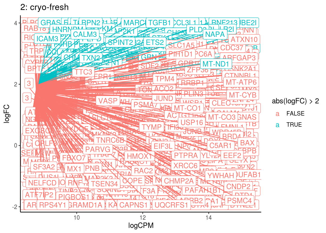
## Cluster: 2 Contrast: cryo-fresh Num genes: 3613 Num DE: 715
##                                    category NGenes Direction       PValue
## 1         GO_MHC_CLASS_II_RECEPTOR_ACTIVITY      6        Up 2.311409e-17
## 2                GO_PEPTIDE_ANTIGEN_BINDING     15        Up 8.873624e-16
## 3 GO_TRANSLATION_ELONGATION_FACTOR_ACTIVITY      7        Up 4.575220e-12
## 4                        GO_ANTIGEN_BINDING     38        Up 6.445838e-12
## 5                           GO_TRNA_BINDING      7        Up 8.778097e-10
## 6   GO_MHC_CLASS_II_PROTEIN_COMPLEX_BINDING     12        Up 8.788584e-08
## 7 GO_STRUCTURAL_CONSTITUENT_OF_CYTOSKELETON     22        Up 1.388469e-07
## 8                          GO_AMIDE_BINDING     68        Up 4.359669e-06
##            FDR
## 1 1.911535e-14
## 2 3.669244e-13
## 3 1.261236e-09
## 4 1.332677e-09
## 5 1.209914e-07
## 6 1.038308e-05
## 7 1.435330e-05
## 8 3.490106e-04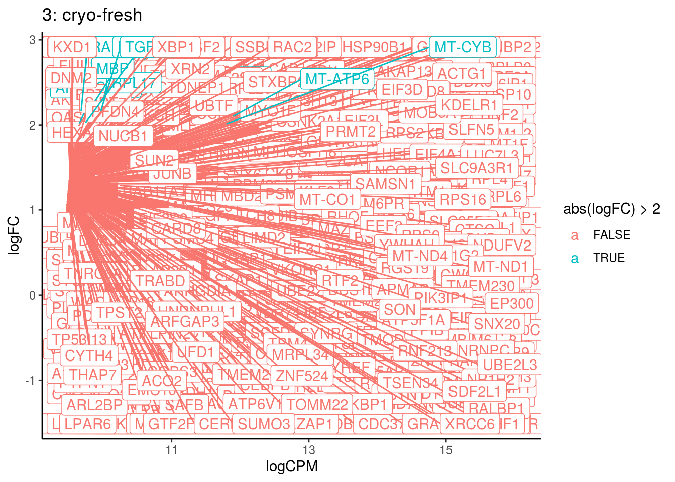
## Cluster: 3 Contrast: cryo-fresh Num genes: 3613 Num DE: 712
##                                     category NGenes Direction       PValue
## 1      GO_STRUCTURAL_CONSTITUENT_OF_RIBOSOME    145        Up 4.275258e-26
## 2            GO_STRUCTURAL_MOLECULE_ACTIVITY    221        Up 6.834261e-18
## 3                            GO_RRNA_BINDING     37        Up 1.286284e-17
## 4                            GO_TRNA_BINDING      7        Up 4.397840e-15
## 5  GO_TRANSLATION_ELONGATION_FACTOR_ACTIVITY      7        Up 4.492579e-14
## 6  GO_STRUCTURAL_CONSTITUENT_OF_CYTOSKELETON     22        Up 2.209793e-08
## 7                 GO_PEPTIDE_ANTIGEN_BINDING     15        Up 1.876794e-06
## 8 GO_TRANSLATION_FACTOR_ACTIVITY_RNA_BINDING     44        Up 1.405468e-05
##            FDR
## 1 3.535638e-23
## 2 2.282420e-15
## 3 2.659393e-15
## 4 7.274027e-13
## 5 6.192271e-12
## 6 2.284373e-06
## 7 1.724565e-04
## 8 1.162322e-03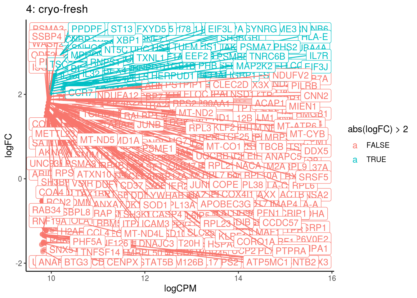
## Cluster: 4 Contrast: cryo-fresh Num genes: 3613 Num DE: 297
##                                     category NGenes Direction       PValue
## 1  GO_TRANSLATION_ELONGATION_FACTOR_ACTIVITY      7        Up 1.262503e-22
## 2      GO_STRUCTURAL_CONSTITUENT_OF_RIBOSOME    145        Up 5.615536e-21
## 3                            GO_TRNA_BINDING      7        Up 4.603774e-20
## 4            GO_STRUCTURAL_MOLECULE_ACTIVITY    221        Up 1.425100e-11
## 5                            GO_RRNA_BINDING     37        Up 7.933755e-10
## 6        GO_FIBROBLAST_GROWTH_FACTOR_BINDING      7        Up 1.502983e-06
## 7 GO_TRANSLATION_FACTOR_ACTIVITY_RNA_BINDING     44        Up 5.704749e-05
##            FDR
## 1 1.044090e-19
## 2 2.322024e-18
## 3 1.269107e-17
## 4 2.946395e-09
## 5 1.312243e-07
## 6 2.071612e-04
## 7 6.739754e-03
Summarize differential expression analysis
# DE genes (per cluster and mean)
#n_de <- lapply(res, function(y) vapply(y, function(x) sum(x$adj.P.Val < 0.05), numeric(1)))
n_de <- lapply(res, function(y) vapply(y, function(x) sum(x$PValue < 0.05), numeric(1)))
n_de_cl <- lapply(res, function(y) vapply(y, function(x) nrow(x), numeric(1)))
mean_n_de <- lapply(n_de, function(x) mean(x))
mean_mean_n_de <- mean(unlist(mean_n_de))/n_genes
min_mean_n_de <- min(unlist(mean_n_de))/n_genes
max_mean_n_de <- max(unlist(mean_n_de))/n_genes

# Genes with lfc > 1
n_genes_lfc1 <- lapply(res, function(y) vapply(y, function(x) sum(abs(x$logFC) > 1), numeric(1)))
mean_n_genes_lfc1 <- mean(unlist(n_genes_lfc1))/n_genes
min_n_genes_lfc1 <- min(unlist(n_genes_lfc1))/n_genes
max_n_genes_lfc1 <- max(unlist(n_genes_lfc1))/n_genes

# DE genes overlap between celltypes (celltype specific de genes)
# Genes are "overlapping" if they are present in all clusters with at least 10% of all cells
de_overlap <- lapply(result, function(x){
  result2 <- x[table(colData(sce)[, celltype]) > ncol(sce) * 0.1]
  de_overlap <- length(Reduce(intersect, result2))
  de_overlap
})

mean_de_overlap <- mean(unlist(de_overlap))/n_genes
min_de_overlap <- min(unlist(de_overlap))/n_genes
max_de_overlap <- max(unlist(de_overlap))/n_genes

#Genes unique to single celltypes
unique_genes_matrix <- NULL
unique_genes <- NULL
cb <- length(names(result[[1]]))
unique_genes <- lapply(result,function(x){
  for( i in 1:cb ){
    unique_genes[i] <-as.numeric(length(setdiff(unlist(x[i]),unlist(x[-i]))))
  }
  unique_genes_matrix <- cbind(unique_genes_matrix, unique_genes)
  unique_genes_matrix
})

unique_genes <- Reduce('cbind', unique_genes)
colnames(unique_genes) <- names(result)
rownames(unique_genes) <- names(result[[1]])

# Relative cluster specificity (unique/overlapping)
rel_spec1 <- NULL
for( i in 1:dim(unique_genes)[2] ){
  rel_spec <- unique_genes[,i]/de_overlap[[i]]
  rel_spec1 <- cbind(rel_spec1,rel_spec)
}

mean_rel_spec <- mean(rel_spec1)
min_rel_spec <- min(rel_spec1)
max_rel_spec <- max(rel_spec1)
Celltype specific DE distributions
How similar is the batch effect between celltypes. Do we have similar logFC distributions or different?
combine_folds <- function(cont_var){
  #extract the contrast of interest and change log2fold colums names to be unique
  B <- res[[cont_var]]
  new_name <- function(p){
    colnames(B[[p]])[3] <- paste0("logFC_", p)
    return(B[[p]][,c(1,3)])
    }
  B_new_names <- lapply(names(B),new_name)
  names(B_new_names) <- names(B)
  #combine log2fold colums
  Folds <- Reduce(function(...){inner_join(..., by="gene")}, B_new_names)
}

all_folds <- lapply(cs, combine_folds)

#define pannels for pairs() function
panel.cor <- function(x, y, digits = 2, cex.cor){
  usr <- par("usr"); on.exit(par(usr))
  par(usr = c(0, 1, 0, 1))
  r <- abs(cor(x, y))
  txt <- format(c(r, 0.123456789), digits=digits)[1]
  test <- cor.test(x,y)
  Signif <- ifelse(round(test$p.value, 3) < 0.001,
                   "p<0.001",
                   paste("p=",round(test$p.value,3)))
  text(0.5, 0.25, paste("r=",txt), cex = 3)
  text(.5, .75, Signif, cex = 3)
}

panel.smooth <- function (x, y, col = "blue", bg = NA, pch = 18, cex = 1.5,
                          col.smooth = "red", span = 2/3, iter = 3, ...){
  points(x, y, pch = pch, col = col, bg = bg, cex = cex)
  ok <- is.finite(x) & is.finite(y)
  if( any(ok) )
    lines(stats::lowess(x[ok], y[ok], f = span, iter = iter),
          col = col.smooth, ...)
}

panel.hist <- function(x, ...){
  usr <- par("usr"); on.exit(par(usr))
  par(usr = c(usr[1:2], 0, 1.5) )
  h <- hist(x, plot = FALSE)
  breaks <- h$breaks
  nB <- length(breaks)
  y <- h$counts
  y <- y/max(y)
  rect(breaks[-nB], 0, breaks[-1], y, col="cyan", ...)
}
#plot correlations
lapply(names(all_folds), function(x) pairs(all_folds[[x]][,-1],
                                           lower.panel = panel.smooth,
                                           upper.panel = panel.cor,
                                           diag.panel = panel.hist, main = x))
## [[1]]
## NULL
#extract correlation coefficients
# correlation coefficients from celltype specific gege logFC
lfc_cor_list <-lapply(names(all_folds), function(com){
exclude <- which(table(colData(sce)[,celltype]) < 100)
r <- cor(all_folds[[com]][, -c(1, (exclude + 1))])
mean_r <- (sum(r) - ncol(r))/ (ncol(r)^2 - ncol(r))
})
mean_lfc_cor <- mean(unlist(lfc_cor_list))Batch categorization
How does the batch effect manifest? Can we describe it by “simple” mean shifts of expression levels for some genes for all the cells in a given celltype and batch? Can we “remove” the batch effcet using a linear model with batch, batch and celltype or batch and celltype interacting?
#Visualize different models
vis_type <- function(dim_red){
  g <- visGroup(sce, batch, dim_red = dim_red) +
    ggtitle("unadjusted")
  g1 <- visGroup(sce, batch, dim_red = paste0(dim_red, "_Xadj1")) +
    ggtitle("constant batch effect")
  g2 <- visGroup(sce, batch, dim_red = paste0(dim_red, "_Xadj2")) +
    ggtitle("constant batch effect, different ct composition")
  g3 <- visGroup(sce, batch, dim_red = paste0(dim_red, "_Xadj3")) +
    ggtitle("celltype and batch effect interact")
  do.call("grid.arrange", c(list(g, g1, g2, g3), ncol = 2))
}
PCA
vis_type("PCA")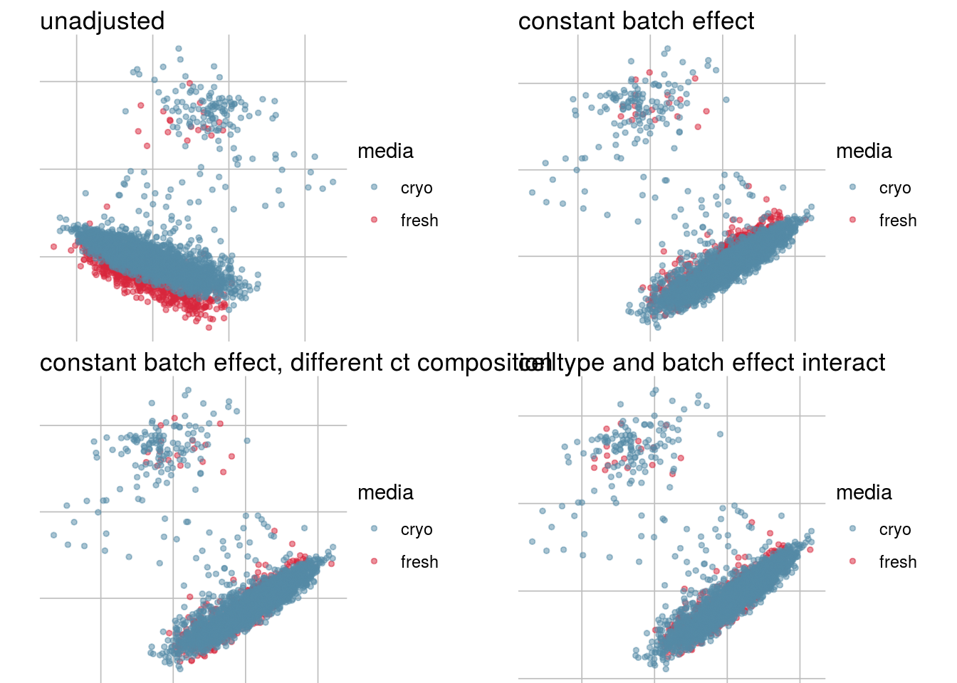
UMAP
vis_type("UMAP")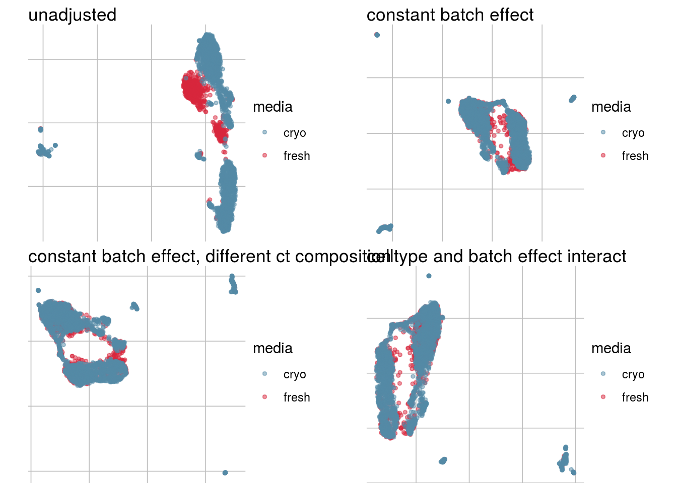
Cellspecific Mixing Score
# #Cellspecific Mixing score (Batch effect strength after "removal")
visHist(sce, metric = c("cms", "cms.Xadj1", "cms.Xadj2", "cms.Xadj3"), prefix = FALSE)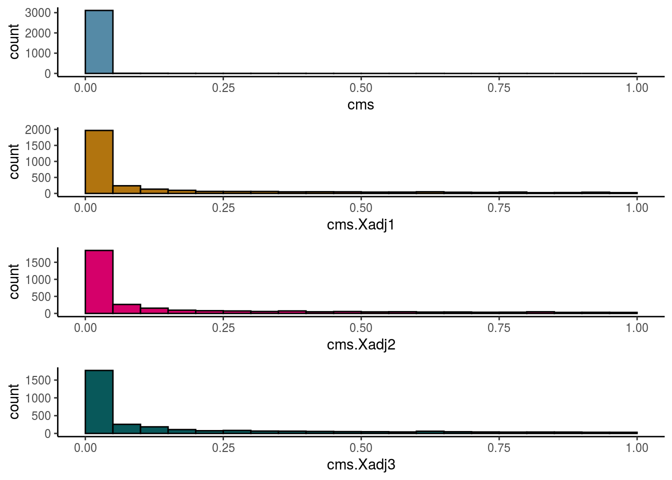
visIntegration(sce, metric = "cms", metric_name = "cms")## Picking joint bandwidth of 0.0163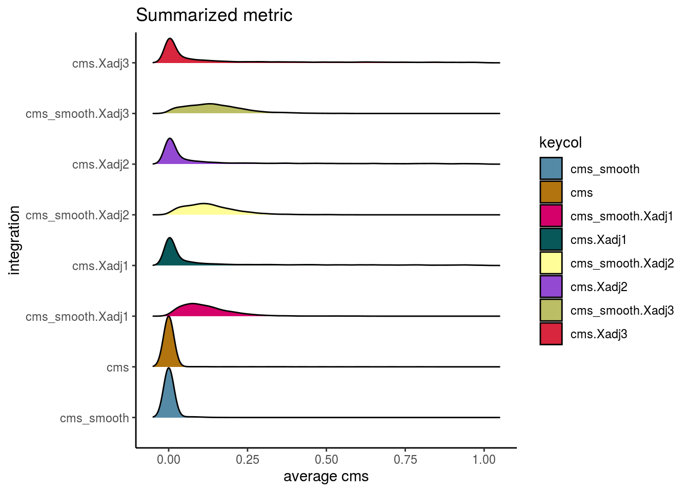
Simulation parameter
Extract parameter to use as input into simualation
#percentage of batch affected genes
cond <- gsub("-.*", "", names(n_de))
cond <- c(cond, unique(gsub(".*-", "", names(n_de))))
cond <- unique(cond)
de_be_tab <- n_de %>% bind_cols()
de_cl_tab <- n_de_cl %>% bind_cols()

de_be <- cond %>% map(function(x){
  de_tab <- de_be_tab[, grep(x, colnames(de_be_tab))]
  de_be <- rowMeans(de_tab)
}) %>% bind_cols() %>% set_colnames(cond)

n_cl <- cond %>% map(function(x){
  cl_tab <- de_cl_tab[, grep(x, colnames(de_cl_tab))]
  de_cl <- rowMeans(cl_tab)
}) %>% bind_cols() %>% set_colnames(cond)


p_be <- de_be/n_cl
mean_p_be <- mean(colMeans(p_be))
min_p_be <- min(colMins(as.matrix(p_be)))
max_p_be <- max(colMaxs(as.matrix(p_be)))
sd_p_be <- mean(colSds(as.matrix(p_be)))
if(is.na(sd_p_be)){ sd_p_be <- 0 }


#### Percentage of celltype specific genes "p_ct"
n_de_unique <- lapply(result,function(x){
  de_genes <- unlist(x) %>% unique() %>% length()
  de_genes <- de_genes/length(x)
}) %>% bind_cols()


rel_spec2 <- NULL
for(i in 1:length(de_overlap)){
  rel_spec <- de_overlap[[i]]/mean(n_de[[i]][table(colData(sce)[, celltype]) > dim(expr)[2] * 0.1])
  rel_spec2 <- cbind(rel_spec2, rel_spec)
}

mean_p_ct <- 1 - mean(rel_spec2)
max_p_ct <- 1 - min(rel_spec2)
min_p_ct <- 1 - max(rel_spec2)
sd_p_ct <- sd(rel_spec2)
if(is.na(sd_p_ct)){ sd_p_ct <- 0 }

# Logfold change
#logFoldchange batch effect distribution
mean_lfc_cl <- lapply(res, function(y) vapply(y, function(x){
  #de_genes <- which(x$adj.P.Val < 0.05)
  de_genes <- which(x$adj.PValue < 0.05)
  mean_de <- mean(abs(x[, "logFC"]))}
  , numeric(1))) %>% bind_cols()

mean_lfc_be <- mean(colMeans(mean_lfc_cl, na.rm = TRUE))
min_lfc_be <- min(colMins(as.matrix(mean_lfc_cl), na.rm = TRUE))
max_lfc_be <- max(colMaxs(as.matrix(mean_lfc_cl), na.rm = TRUE))
Summarize batch effect
- Batch size
- Celltype specificity
- “Batch genes”
- batch type
#Size? How much of the variance can be attributed to the batch effect?
size <- data.frame("batch_genes_1per" = n_batch_gene,       # 1.variance partition
                   "batch_genes_10per" = n_batch_gene10,
                   "celltype_gene_1per" = n_celltype_gene,
                   "relative_batch_celltype" = n_rel,
                   "mean_var_batch" = m_batch,
                   "mean_var_celltype" = m_celltype,
                   "rel_mean_ct_batch" = m_rel,
                   "mean_cms" = mean_cms,                    #2.cms
                   "n_cells_cms_0.01" = n_cms_0.01,
                   "mean_mean_n_de_genes" = mean_mean_n_de,  #3.de genes
                   "max_mean_n_de_genes" = max_mean_n_de,
                   "min_mean_n_de_genes" = min_mean_n_de,
                   "mean_n_genes_lfc1" = mean_n_genes_lfc1,
                   "min_n_genes_lfc1" = min_n_genes_lfc1,
                   "max_n_genes_lfc1" = max_n_genes_lfc1,
                   "n_cells_total" = ncol(sce),              #4.general
                   "n_genes_total" = nrow(sce))


#Celltype-specificity? How celltype/cluster specific are batch effects?
# Differences in size, distribution or abundance? Do we find correlations between lfcs,
# overlap in de genes, pathways? Interaction between ct and be?
celltype <- data.frame('mean_rel_abund_diff' = mean_rel_abund_diff, #1.abundance
                       'min_rel_abund_diff' = min_rel_abund_diff,
                       'max_rel_abund_diff' = max_rel_abund_diff,
                       "celltype_var_cms" = var_cms,                 #2.size/strength
                       "mean_de_overlap" = mean_de_overlap,
                       "min_de_overlap" = min_de_overlap,
                       "max_de_overlap" = max_de_overlap,
                       "mean_rel_cluster_spec"= mean_rel_spec,
                       "min_rel_cluster_spec"= min_rel_spec,
                       "max_rel_cluster_spec"= max_rel_spec,
                       "mean_lfc_cor" = mean_lfc_cor )


sim <- data.frame("mean_p_be" = mean_p_be,
                  "max_p_be" = max_p_be,
                  "min_p_be" = min_p_be,
                  "sd_p_be" = sd_p_be,
                  "mean_lfc_be" = mean_lfc_be,
                  "min_lfc_be" = min_lfc_be,
                  "max_lfc_be" = max_lfc_be,
                  "mean_p_ct"= mean_p_ct,
                  "min_p_ct"= min_p_ct,
                  "max_p_ct"= max_p_ct,
                  "sd_p_ct" = sd_p_ct)


summary <- cbind(size, celltype, sim) %>% set_rownames(dataset_name)

### -------------- save summary object ----------------------###
saveRDS(summary, file = outputfile)sessionInfo()## R version 3.6.1 (2019-07-05)
## Platform: x86_64-pc-linux-gnu (64-bit)
## Running under: Ubuntu 16.04.6 LTS
##
## Matrix products: default
## BLAS: /home/aluetg/R/lib/R/lib/libRblas.so
## LAPACK: /home/aluetg/R/lib/R/lib/libRlapack.so
##
## locale:
## [1] LC_CTYPE=en_US.UTF-8 LC_NUMERIC=C
## [3] LC_TIME=en_US.UTF-8 LC_COLLATE=en_US.UTF-8
## [5] LC_MONETARY=en_US.UTF-8 LC_MESSAGES=en_US.UTF-8
## [7] LC_PAPER=en_US.UTF-8 LC_NAME=C
## [9] LC_ADDRESS=C LC_TELEPHONE=C
## [11] LC_MEASUREMENT=en_US.UTF-8 LC_IDENTIFICATION=C
##
## attached base packages:
## [1] grid parallel stats4 stats graphics grDevices utils
## [8] datasets methods base
##
## other attached packages:
## [1] readr_1.3.1 ggrepel_0.8.2
## [3] CAMERA_1.42.0 xcms_3.8.2
## [5] MSnbase_2.12.0 ProtGenerics_1.18.0
## [7] mzR_2.20.0 Rcpp_1.0.3
## [9] cowplot_1.0.0 scran_1.14.6
## [11] gridExtra_2.3 ComplexHeatmap_2.2.0
## [13] stringr_1.4.0 dplyr_0.8.5
## [15] tidyr_1.0.2 here_0.1
## [17] jcolors_0.0.4 purrr_0.3.3
## [19] variancePartition_1.16.1 scales_1.1.0
## [21] foreach_1.4.8 limma_3.42.2
## [23] CellMixS_1.2.4 kSamples_1.2-9
## [25] SuppDists_1.1-9.5 scater_1.14.6
## [27] ggplot2_3.3.0 CellBench_1.2.0
## [29] tibble_2.1.3 magrittr_1.5
## [31] SingleCellExperiment_1.8.0 SummarizedExperiment_1.16.1
## [33] DelayedArray_0.12.2 BiocParallel_1.20.1
## [35] matrixStats_0.55.0 Biobase_2.46.0
## [37] GenomicRanges_1.38.0 GenomeInfoDb_1.22.0
## [39] IRanges_2.20.2 S4Vectors_0.24.3
## [41] BiocGenerics_0.32.0
##
## loaded via a namespace (and not attached):
## [1] tidyselect_1.0.0 lme4_1.1-21 RSQLite_2.2.0
## [4] htmlwidgets_1.5.1 munsell_0.5.0 codetools_0.2-16
## [7] preprocessCore_1.48.0 statmod_1.4.34 withr_2.1.2
## [10] colorspace_1.4-1 knitr_1.28 rstudioapi_0.11
## [13] robustbase_0.93-5 mzID_1.24.0 labeling_0.3
## [16] GenomeInfoDbData_1.2.2 farver_2.0.3 bit64_0.9-7
## [19] rprojroot_1.3-2 vctrs_0.2.4 xfun_0.12
## [22] BiocFileCache_1.10.2 R6_2.4.1 doParallel_1.0.15
## [25] ggbeeswarm_0.6.0 clue_0.3-57 rsvd_1.0.3
## [28] locfit_1.5-9.1 bitops_1.0-6 assertthat_0.2.1
## [31] nnet_7.3-13 beeswarm_0.2.3 gtable_0.3.0
## [34] affy_1.64.0 rlang_0.4.5 GlobalOptions_0.1.1
## [37] splines_3.6.1 acepack_1.4.1 impute_1.60.0
## [40] checkmate_2.0.0 BiocManager_1.30.10 yaml_2.2.1
## [43] reshape2_1.4.3 backports_1.1.5 Hmisc_4.3-1
## [46] MassSpecWavelet_1.52.0 RBGL_1.62.1 tools_3.6.1
## [49] ellipsis_0.3.0 affyio_1.56.0 gplots_3.0.3
## [52] RColorBrewer_1.1-2 ggridges_0.5.2 plyr_1.8.6
## [55] base64enc_0.1-3 progress_1.2.2 zlibbioc_1.32.0
## [58] RCurl_1.98-1.1 prettyunits_1.1.1 rpart_4.1-15
## [61] GetoptLong_0.1.8 viridis_0.5.1 cluster_2.1.0
## [64] colorRamps_2.3 data.table_1.12.8 circlize_0.4.8
## [67] RANN_2.6.1 pcaMethods_1.78.0 packrat_0.5.0
## [70] hms_0.5.3 evaluate_0.14 pbkrtest_0.4-8.6
## [73] XML_3.99-0.3 jpeg_0.1-8.1 shape_1.4.4
## [76] compiler_3.6.1 KernSmooth_2.23-16 ncdf4_1.17
## [79] crayon_1.3.4 minqa_1.2.4 htmltools_0.4.0
## [82] mgcv_1.8-31 Formula_1.2-3 lubridate_1.7.4
## [85] DBI_1.1.0 dbplyr_1.4.2 MASS_7.3-51.5
## [88] rappdirs_0.3.1 boot_1.3-24 Matrix_1.2-18
## [91] cli_2.0.2 vsn_3.54.0 gdata_2.18.0
## [94] igraph_1.2.4.2 pkgconfig_2.0.3 foreign_0.8-76
## [97] MALDIquant_1.19.3 vipor_0.4.5 dqrng_0.2.1
## [100] multtest_2.42.0 XVector_0.26.0 digest_0.6.25
## [103] graph_1.64.0 rmarkdown_2.1 htmlTable_1.13.3
## [106] edgeR_3.28.1 DelayedMatrixStats_1.8.0 listarrays_0.3.1
## [109] curl_4.3 gtools_3.8.1 rjson_0.2.20
## [112] nloptr_1.2.2.1 lifecycle_0.2.0 nlme_3.1-145
## [115] BiocNeighbors_1.4.2 fansi_0.4.1 viridisLite_0.3.0
## [118] pillar_1.4.3 lattice_0.20-40 httr_1.4.1
## [121] DEoptimR_1.0-8 survival_3.1-11 glue_1.3.1
## [124] png_0.1-7 iterators_1.0.12 bit_1.1-15.2
## [127] stringi_1.4.6 blob_1.2.1 BiocSingular_1.2.2
## [130] latticeExtra_0.6-29 caTools_1.18.0 memoise_1.1.0
## [133] irlba_2.3.3