library(scran)
library(dplyr)
library(tidyr)
library(ggplot2)
library(scuttle)
library(scater)
library(DT)
library(patchwork)
library(SingleCellExperiment)
library(stringr)
library(gridExtra)data_viz
Data viz
Different ways to look at the preprocessed dataset
Preamble
Data
sce <- readRDS(file.path("..", "data", "sce_all_metadata_genes.rds"))
meta_dat <- read.csv(file.path("..", "data", "metadata.csv"),
                     sep = "\t", row.names = 1)

# major celltypes
sce$ct_broad <- sce$cell_type_name |> forcats::fct_collapse(
  "capillary" = c("1 capillary1", "2 capillary2"),
  "precollector" = c("3 precollector1", "4 precollector2"),
  "collector" = c("5 collector"),
  "valve" = c("6 valve"),
  "prolieferative" = c("7 proliferative"))


#colours to correspond to shinycell
cList = list("cell_type_name" = c("#A6CEE3","#99CD91","#B89B74",
                                  "#F06C45","#ED8F47","#825D99","#B15928"),
             "tissue" = c("#A6CEE3","#F06C45","#B15928"),
             "donor" = c("#A6CEE3","#99CD91","#B89B74",
                         "#F06C45","#ED8F47","#825D99","#B15928"))
names(cList[["cell_type_name"]]) <- c("1 capillary1","2 capillary2","3 precollector1","4 precollector2","5 collector","6 valve","7 proliferative")
names(cList[["tissue"]]) <- c("fat","mixed","skin")
names(cList[["donor"]]) <- c("1.0","2.0","3.0","4.0","5.0","6.0","7.0")
cells per ct
table(sce$tissue)
  fat mixed  skin
7300 4705 9369 table(sce$donor)
 1.0  2.0  3.0  4.0  5.0  6.0  7.0
3902 2773 1247 631 4705 3647 4469 table(sce$cell_type_name)
   1 capillary1    2 capillary2 3 precollector1 4 precollector2     5 collector
           6023            1156            5407            6041            1105
        6 valve 7 proliferative
1555 87 table(sce$ct_broad)
     capillary   precollector      collector          valve prolieferative
7179 11448 1105 1555 87 table(sce$ct_broad, sce$tissue)
                  fat mixed skin
  capillary      2206  1412 3561
  precollector   3999  2663 4786
  collector       613   249  243
  valve           449   371  735
prolieferative 33 10 44table(sce$cell_type_name, sce$tissue)
                   fat mixed skin
  1 capillary1    1748  1167 3108
  2 capillary2     458   245  453
  3 precollector1 1750  1163 2494
  4 precollector2 2249  1500 2292
  5 collector      613   249  243
  6 valve          449   371  735
  7 proliferative   33    10   44
Data viz
Umap split by tissue
sce_fat <- sce[,sce$tissue %in% "fat"]
sce_skin <- sce[,sce$tissue %in% "skin"]
sce_mixed <- sce[,sce$tissue %in% "mixed"]

p1 <- plotReducedDim(sce_fat, dimred="umap",
                     colour_by="cell_type_name",
                     point_size = 0.8) +
  ggtitle("fat") +
  scale_color_manual(values = cList[["cell_type_name"]])
Scale for colour is already present.
Adding another scale for colour, which will replace the existing scale.p2 <- plotReducedDim(sce_skin, dimred="umap",
colour_by="cell_type_name",
point_size = 0.8) +
ggtitle("skin") +
scale_color_manual(values = cList[["cell_type_name"]])Scale for colour is already present.
Adding another scale for colour, which will replace the existing scale.p3 <- plotReducedDim(sce_mixed, dimred="umap",
colour_by="cell_type_name",
point_size = 0.8) +
ggtitle("mixed") +
scale_color_manual(values = cList[["cell_type_name"]])Scale for colour is already present.
Adding another scale for colour, which will replace the existing scale.wrap_plots(list("skin" = p2,
"mixed" = p3,
"fat" = p1), nrow = 1) +
plot_layout(guides = "collect") &
theme(legend.position = "bottom")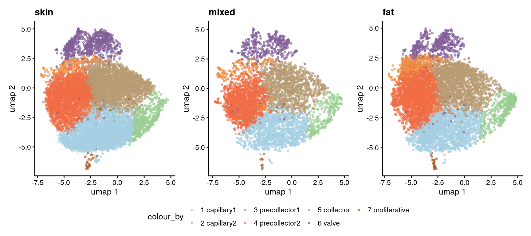
Umap before after integration
no_int <- calculateUMAP(reducedDims(sce)[["logcounts.scaled.pca"]],transposed = T)
reducedDims(sce)[["logcounts.scaled.umap"]] <- no_int


p1 <- plotReducedDim(sce, dimred="umap", colour_by="donor", point_size = 0.8) +
  ggtitle("after") +
  scale_color_manual(values = cList[["donor"]])
Scale for colour is already present.
Adding another scale for colour, which will replace the existing scale.p2 <- plotReducedDim(sce, dimred="logcounts.scaled.umap", colour_by="donor", point_size = 0.8) +
ggtitle("before") +
scale_color_manual(values = cList[["donor"]])Scale for colour is already present.
Adding another scale for colour, which will replace the existing scale.wrap_plots(list("before" = p2,
"after" = p1), nrow = 1) +
plot_layout(guides = "collect") &
theme(legend.position = "bottom")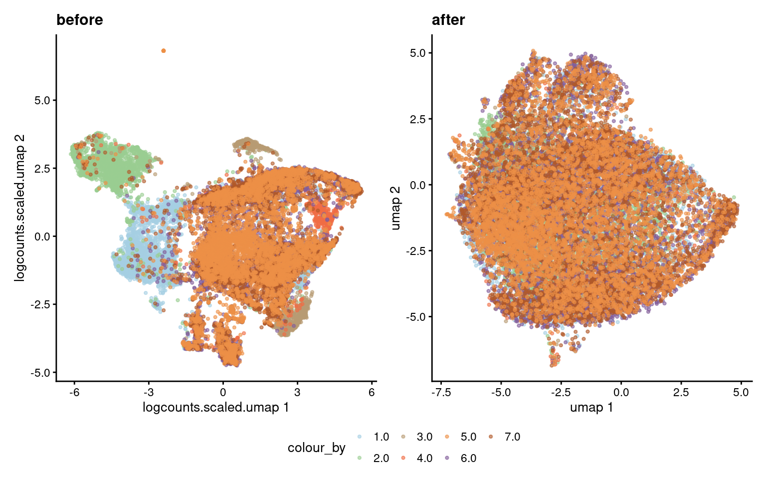
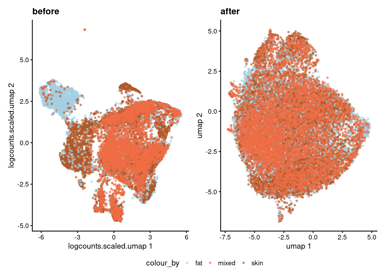
coloured by tissue
p1 <- plotReducedDim(sce, dimred="umap", colour_by="tissue", point_size = 0.8) +
  ggtitle("after") +
  scale_color_manual(values = cList[["tissue"]])
Scale for colour is already present.
Adding another scale for colour, which will replace the existing scale.p2 <- plotReducedDim(sce, dimred="logcounts.scaled.umap", colour_by="tissue", point_size = 0.8) +
ggtitle("before") +
scale_color_manual(values = cList[["tissue"]])Scale for colour is already present.
Adding another scale for colour, which will replace the existing scale.wrap_plots(list("before" = p2,
"after" = p1), nrow = 1) +
plot_layout(guides = "collect") &
theme(legend.position = "bottom")